Abstract
The date of a historical document, if it was published, can be recognized through the date of its preface or copyright page. However, dating an unpublished manuscript is much more difficult. In the case of old Hangeul documents, various linguistic features can be used to estimate the approximate date of the document, but as the number of features increases, the task tends to go beyond the purview of an individual human researcher, and become more appropriate to AI. This paper shows how artificial neural networks can be trained to estimate the date of documents using material whose date is known. For this purpose, various kinds of neural networks are examined: Bag-of-words model, CNN, RNN and Transformer. In addition, these models can be further sub-divided: unigram or bigram, character(syllable)-based or grapheme(phoneme)-based. After trained on documents with known dates, these models are applied to new (unseen) data, and the results are evaluated.
-
Keywords: deep learning, neural network, dating, historical document, inference
1. SETTING THE SCENE
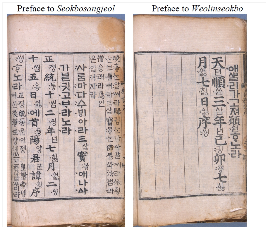
Among materials on the history of the Korean language, printed editions with colophons have been actively utilized because their publication dates are clear. For example, the prefaces of
Seokbosangjeol and
Weolinseokbo contain Chinese era names, so these indicate the years of compilation or publishing (
Figure 1).
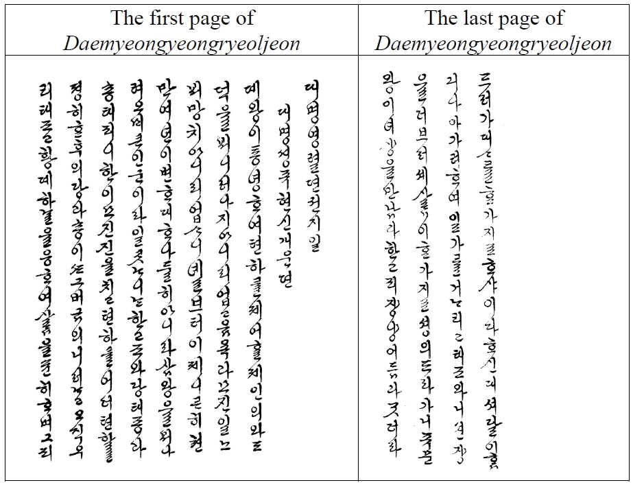
On the other hand, manuscripts have generally been used less frequently in research on the history of the Korean language due to their unclear dates. For example,
Daemyeongyeongryeoljeon, a manuscript novel, has no indication of the year of writing (
Figure 2).
Nevertheless, given the substantial volume of manuscript materials, it would be beneficial to estimate their dates in some way so that they can be utilized in research on the history of the Korean language.
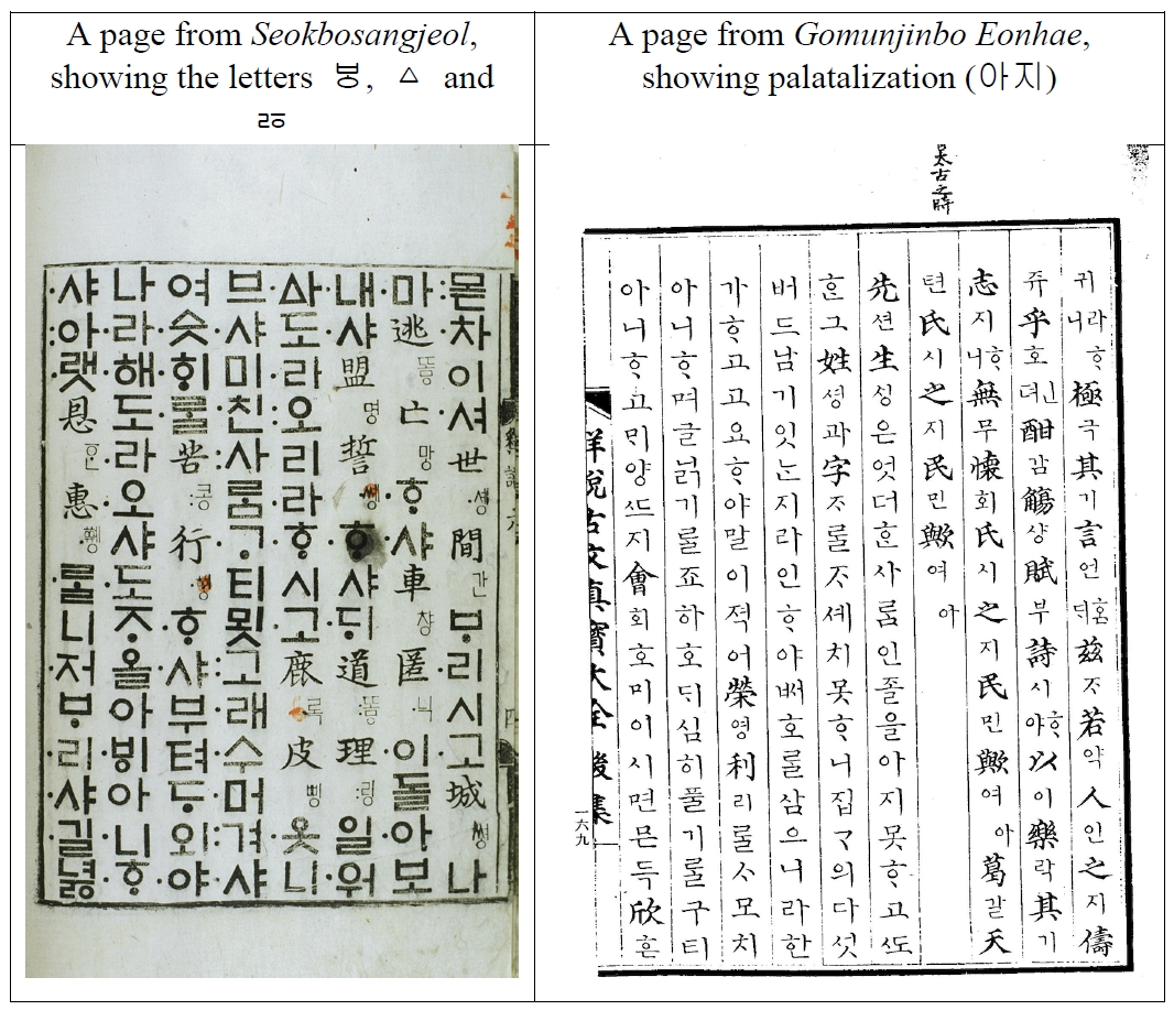
Linguists can use linguistic clues (e.g. consonants ㅸ, ㅿ, ㅭ or phonological phenomena such as palatalization 아디>아지) to estimate the approximate dates of these documents (
Figure 3).
However, there are enormous number of linguistic features which can be used as clues for estimating the date, which cannot be considered by human researchers in their entirety, so they generally use very small part of these evidences. In such cases, machines (especially deep learning models) are excellent in taking all these features into account, so using deep learning for this task seems to be promising.
Many linguists and literary scholars are not familiar with machine learning concepts and techniques. Some of them think that they need not know much about machine learning, expecting that AI will solve their problems. However, when experimenting with machine learning to solve a task, one should make many decisions (about e.g. models, hyperparameters, etc.). These decisions require knowledge of machine learning. We need educated guidance in deciding which option to try.
2. PREPARING THE DATA
In order to train a deep learning model, we need many samples, usually several dozens of thousand. The amount of the extant Korean historical documents is fixed. If we set the length of each sample short, we can get many samples. But then we can risk having few clues of the date in a sample. If we set the length of each sample long, we have fewer samples. As a result of some experimenting, I set 300 characters as the length of each sample, which results in about 50 thousand samples (
Table 1).
3. BAG-OF-WORDS UNIGRAM MODEL
As a first rough attempt, I tried a bag-of-words unigram model. ‘Bag-of-words’ means that each sample is considered as a set of tokens, disregarding the order. ‘Unigram’ means that each single character is a basic unit. (Bigram models mean that each pair of characters, as well as each single character, is a basic unit, which will be touched upon later.)
In order to enter each sample into a neural network, it should be represented as a number or a series of numbers (i.e. a vector). This process is called vectorization, embedding or encoding. Several methods of encoding have been invented. I used one-hot encoding. In this encoding scheme, only the most frequent ten thousand characters were considered. Each sample is represented as a vector of ten thousand digits. ‘1’ means that the sample contains the letter, whereas ‘0’ means otherwise. This process is covered at the Text Vectorization Layer.
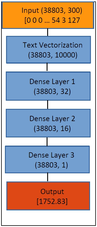
As for the architecture of the neural network (
Figure 4), I used a dense (also called fully connected) network consisting of three dense layers. In Dense Layer 1, the dimensionality of each vector representing a sample is reduced from 10,000 to 32. In Dense Layers 2 and 3, the dimensionality is further reduced to 16 and finally to 1. This final floating number is supposed to correspond to the estimated year of the input sample.
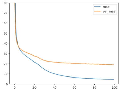
This model was trained for 100 epochs. The 95th epoch showed the best performance (
Figure 5). At this epoch, the losses, i.e. MSE (mean squared error) and MAE (mean absolute error), were as in
Table 2.
The error of about 20 years seems to be promising. Even human experts cannot produce this level of accuracy. They usually estimate at the level of half century. The first very simple model achieved a very good (super-human) result!
4. ADDING REGULARIZATION TO A BAG-OF-WORDS / UNIGRAM MODEL
The above model shows a quite large difference between the training set and the validation set, which means that overfitting is occurring. When overfitting occurs, the model’s performance for new data tends to degrade. Many methods have been created for restricting the model’s power to prevent or alleviate overfitting. The first is layer regularizers, by which the sum of absolute values (L1) or squares (L2) of weights is added to the loss in order to prevent the weights from becoming too large. The second is batch normalization, by which each batch of samples is normalized. The third is dropout, by which a fixed proportion (in our case 0.3) of nodes in each layer is set to zero. In compensation for regularization, I doubled the number of nodes of Dense Layer 1 (32 to 64) and 2 (16 to 32).
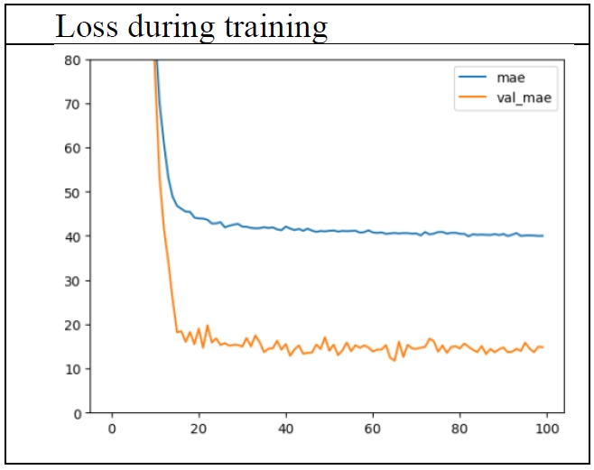
This model was also trained for 100 epochs. The 65th epoch showed the best performance (
Figure 6). At this epoch, the losses were as in
Table 3.
The performance in the test set is most important, because it shows the estimated error rate for new data. The error of 15.85 years seems very good, much better than the previous result of about 20 years. But it seems odd that the performance in the test set is better than that in the training set.
5. INCREASING THE MODEL’S POWER
The bizarre phenomenon in which the performance in the test set is better than that in the training set, may be due to the lack of power of the model, compared to the added regularization. So I doubled again the number of nodes of Dense Layer 1 (64 to 128) and 2 (32 to 64), and decreased the dropout rate from 0.3 to 0.2.
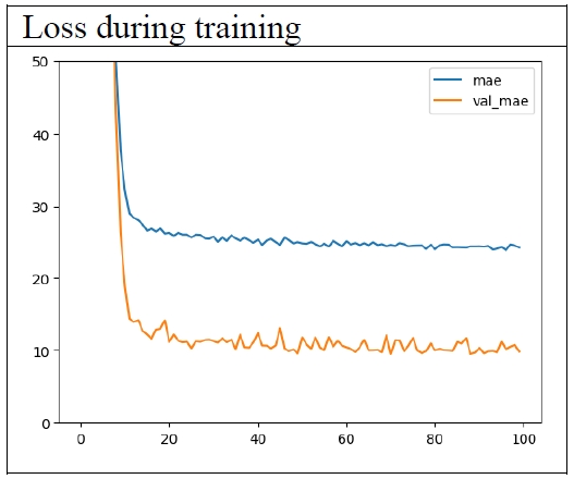
This model was also trained for 100 epochs. The 67th epoch showed the best performance (
Figure 7). At this epoch, the losses were as in
Table 4.
The bizarre phenomenon in which the performance in the test set is better than that in the training set, still appears. The good news is that the error has decreased to 11.4 years.
6. BAG-OF-WORDS / BIGRAM MODEL
In the above experiment, each single character was considered as a basic unit. Of course, whether a particular single character appears in a sample can be a good indicator of the date of the sample, but in addition, whether a particular sequence of two consecutive characters appears in a sample can also be a good clue. For example, the sequence of 아 and 비 can be considered as an evidence that umlaut has not yet occurred in this sample, whereas the sequence of 애 and 비 can be an (although not perfect) indicator of umlaut.
Therefore, I experimented with bigrams. The library Keras provides the option ‘ngrams=2’ when generating the object of the class TextVectorization. As we should consider bigrams as well as unigrams, I increased the number of token types from 10,000 to 20,000. The architecture of the model is the same as the previous one. In Dense Layer 1, the dimensionality of each sample is reduced from 20,000 to 128, which is further reduced to 64 and to 1 in Dense Layer 2 and 3 respectively. I added the three kinds of regularization to Dense Layer 1 and 2.
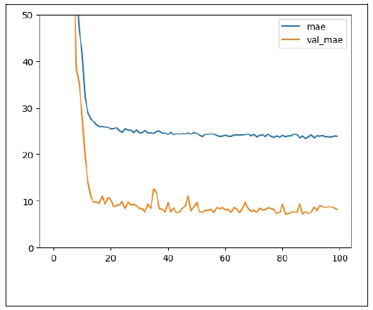
This model was also trained for 100 epochs. The 83th epoch showed the best performance (
Figure 8). At this epoch, the losses were as in
Table 5.
The bizarre phenomenon in which the performance in the test set is better than that in the training set, still appears. The good news is that the error has decreased to 8.54 years.
7. CNN MODEL
In the area of computer vision, CNN (convolutional neural network) models have been popular. In order to extract local patterns from 2-dimensional image, CNN uses a small 2-D window. As a text is a 1-dimensional sequence, 1-D window is used in CNN models for textual data.
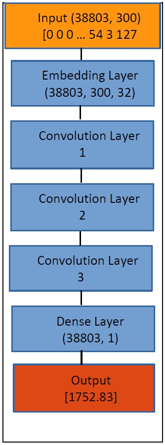
In order to enter a sample (1-D sequence of tokens), we should encode each token (character) as a vector. This task is covered in Embedding Layer (
Figure 9). In our case, each character was encoded as a 32-dimensional vector. In Convolution Layer 1, a window of size 3 moves from the beginning to the end of a sample, and extracts information. Due to this process, the dimensionality of each sample is reduced from 300 to 298. In the following two Convolution Layers, the same process is repeated, and the dimensionality is further reduced to 296 and to 294. In Convolution Layer 3, each node corresponds to seven tokens in the input sample. In Global Pooling Layer, all the information is synthesized. In Dense Layer, each sample is reduced to one floating point number, which is the estimated year of the sample.
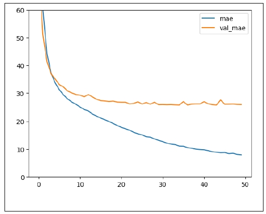
This model was trained for 50 epochs. The 24th epoch showed the best performance (
Figure 10). At this epoch, the losses were as in Table
Overfitting occurs, as the difference between the performance in the training set and that in the test set is quite large. The error in the test set is about 27 years, which is not so good.
8. RNN MODEL
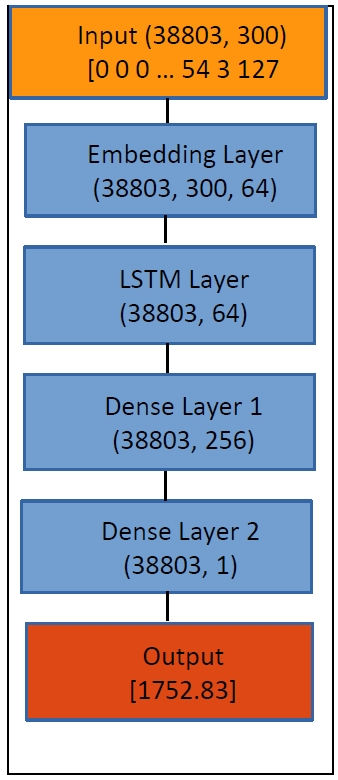
CNN is appropriate for extracting position-invariant information. ‘Position-invariant’ means that it doesn’t matter where in the input sample a feature is located. This accords with image data, but not with textual data, in which the positional information matters. For textual data, RNN (recurrent neural network) is better suited than CNN. Among several variants of RNN, LSTM performs very well, so I chose that (
Figure 11).
Just like CNN, each token is encoded as a vector of 64 numbers in Embedding Layer. Next, in the bidirectional LSTM Layer, each sample is summarized as a single vector, going forward and backward inside the sample. Finally, in Dense Layers, each sample outputs a single number, the estimated year.
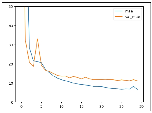
This model was trained for 30 epochs. The 25th epoch showed the best performance (
Figure 12). At this epoch, the losses were as in
Table 7.
Overfitting doesn’t occur, as the difference between the performance in the training set and that in the test set is small. The error in the test set is about 11 years, which is the best record so far.
9. DECOMPOSITION INTO GRAPHEMES
In Hangeul, a character consists of three graphemes (an onset, a nucleus and a coda). The information of which grapheme follows which grapheme (especially across syllable/character boundaries) is very important, and can contribute to the estimation of the date. Therefore, I experimented by decomposing each character into graphemes.
Each sample consists of up to 300 characters, and when decomposed into graphemes, the length (number of graphemes) of a sample increases. The longest sample was 933 tokens long. The number of the kinds of characters was 13737, but when decomposed into graphemes, the number of the kinds of tokens decreases to 9805. Among these 9805 tokens, only the 5000 most frequent tokens are considered.
The CNN unigram model showed the MAE 20.73 years, whereas the RNN model showed the MAE 16.00 years.
The importance of bigram models increases when using grapheme decomposition. For example, the sequence of ㄷ and ㅣ can be considered as an evidence that palatalization has not yet occurred in this sample, whereas the sequence of ㅈ and ㅣ can be an (although not perfect) indicator of palatalization. I only considered the 20,000 most frequent unigrams and bigrams. The MAE of the CNN model was 21.55 years, the RNN model 13.59 years, the Bag-of-words model 10.51 years, and the Bag-of-words model using TF-IDF 9.87 years. These models showed small increases in performance, but the margins are not so large.
10. TRANSFORMER MODEL
When an input sample is a sequence of tokens and the order of tokens matters, the traditional approach to capturing these sequential patterns has been RNN, including LSTM. But as RNN must process input tokens one by one and it is impossible to parallelize, it takes enormous time to train an RNN model. The transformer model, released in 2017, captures the dependency patterns among input tokens through attention mechanism and it is possible to parallelize, it takes much less time to train a transformer model. Therefore, I experimented with a transformer model, using the TransformerEncoder layer in the library Keras. The architecture of the model is almost identical to the RNN model, only replacing the LSTM layer with the TransformerEncoder layer.
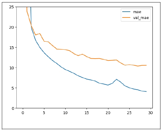
This model was trained for 30 epochs. The 25th epoch showed the best performance (
Figure 13). At this epoch, the losses were as in
Table 8.
Overfitting doesn’t occur, as the difference between the performance in the training set and that in the test set is not so large. The error in the test set is about 10.84 years, which is the best record so far.
11. HEATMAP
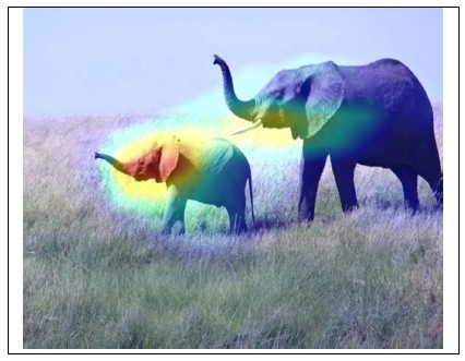
A heatmap is a plot showing the activation level of each node in a neural network. In the case of images, a node corresponds to a pixel or a tiny local set of pixels. For example, in an image of an African elephant, pixels corresponding to its trunk are more important than pixels corresponding to the sky, the grass or the body in judging the identity of the object in the image (
Figure 14).
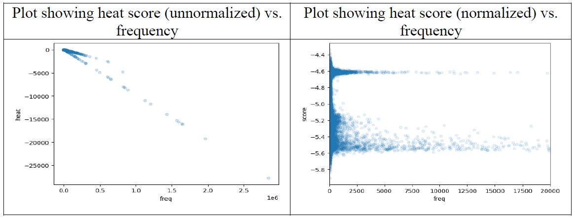
When constructing a heatmap, the nodes in the last convolution layer are considered, and the heat scores are aggregated per each token. The higher the frequency of the token is, the higher the aggregated heat score is, so we need to normalize the effect of frequency.
The following two plots (
Figure 15) show the relationship between each token’s heat score and frequency. Before normalizing, the two shows strong correlation, but after normalized, the effect of frequency is near to zero. (The two peaks in the plot corresponds to unigrams and bigrams.
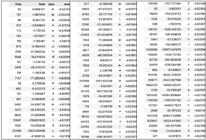
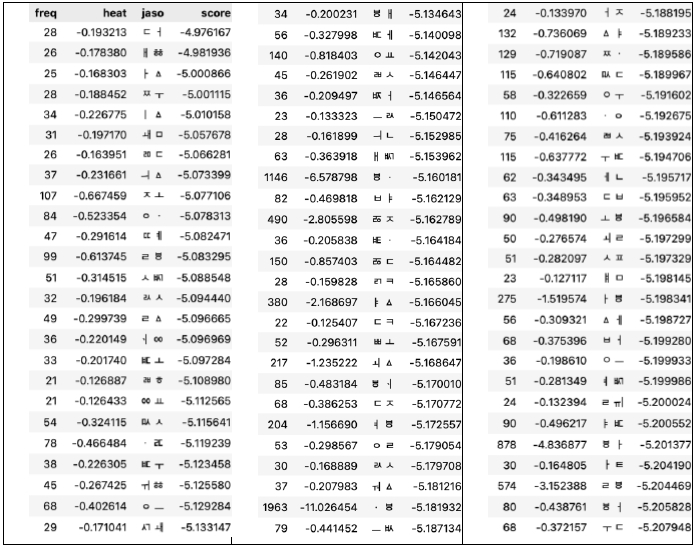
I ordered the tokens (unigrams and bigrams) according to the normalized heat scores (
Tables 9 and
10). As can be seen in these tables, the model pays attention to tokens characteristic to the date of the sample.
12. INFERENCE AND EVALUATION
I applied the LSTM model to documents of the 15th century (
Table 11). The MSE is 163.10 and the MAE is 7.46 years, which shows that the model’s prediction is quite accurate. This result is unsurprising because these documents were seen repeatedly in the training process. Speaking metaphorically, a student can get a high score in a test if the questions were already known to her, which is a matter of course.
More important is the performance when the model is applied to data which were never seen by the model in the training process. For this purpose, I used documents from Jangseogak in the Academy of Korean Studies. These documents are mostly manuscripts, so the precise dates are not known. However, some researchers have been estimating the dates of these documents using linguistic features and historical events recorded in the documents.
Table 12 shows the date of these documents predicted by the LSTM model.
Experts in these documents says that these predictions are quite accurate. Although the predictions as to some very short documents went somewhat wide, most predictions were near the estimation by domain experts.
Table 13 shows the date of these documents predicted by the Transformer model.
The predictions of these two models are quite similar, as can be seen in
Table 14. The MAE between these two predictions is 32.52 years. This shows that the predictions of these two models are quite stable and reliable.
A document can consist of many samples, and the model’s predictions as to samples coming from the same document can vary. The standard deviation of these predictions indicates the homogeneity or heterogeneity of the document. According to the standard deviations,
Cheonjusilui is most homogeneous, whereas
Gyehaebanjeongrok is most heterogeneous, and the two models agree in this respect too (
Tables 12 and
13).
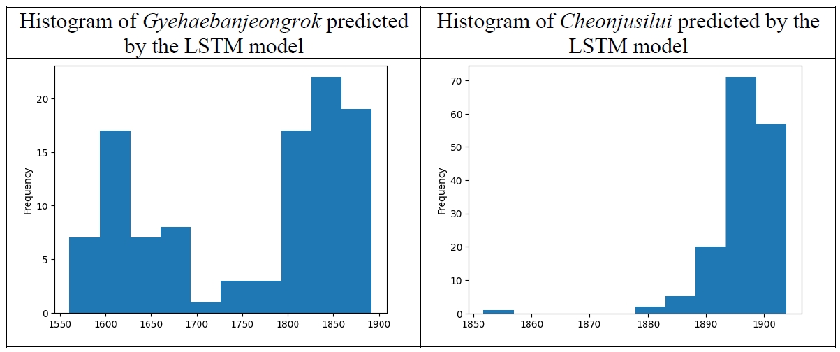
The plots in
Figure 16 are the histograms showing the dates of the samples of
Gyehaebanjeongrok and
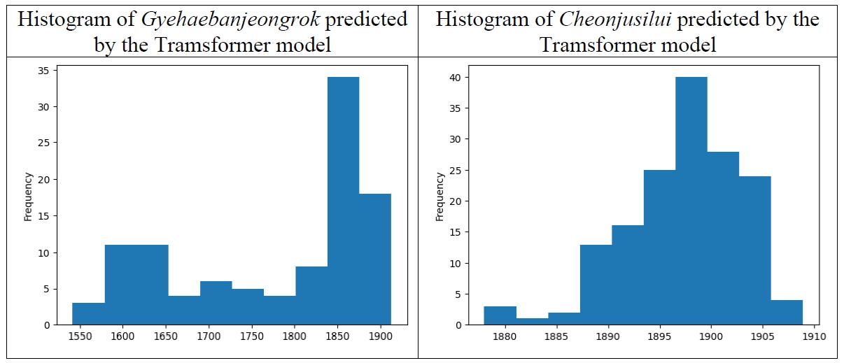
Cheonjusilui predicted by the LSTM model. The samples of
Cheonjusilui are quite homogeneous, whereas the samples
Gyehaebanjeongrok of are divided into two clusters.
This pattern is repeated exactly in
Figure 17, showing the dates of the samples of
Gyehaebanjeongrok and
Cheonjusilui predicted by the Tramsformer model.
13. CONCLUSION
In order to estimate the date of historical documents, I trained several neural network models using document with known dates. As a result of the experiments, the Bag-of-words bigram model, the LSTM model and the Transformer model showed the best results. Whether we use characters (syllables) or graphemes (phonemes) as basic units doesn’t matter so much. It is promising that the LSTM and Transformer models brought forward very similar results. This indicates the stability and reliability of the models. It is also helpful that we can investigate the variability among samples coming from the same document.
Figure 1Prefaces to Seokbosangjeol and Weolinseokbo
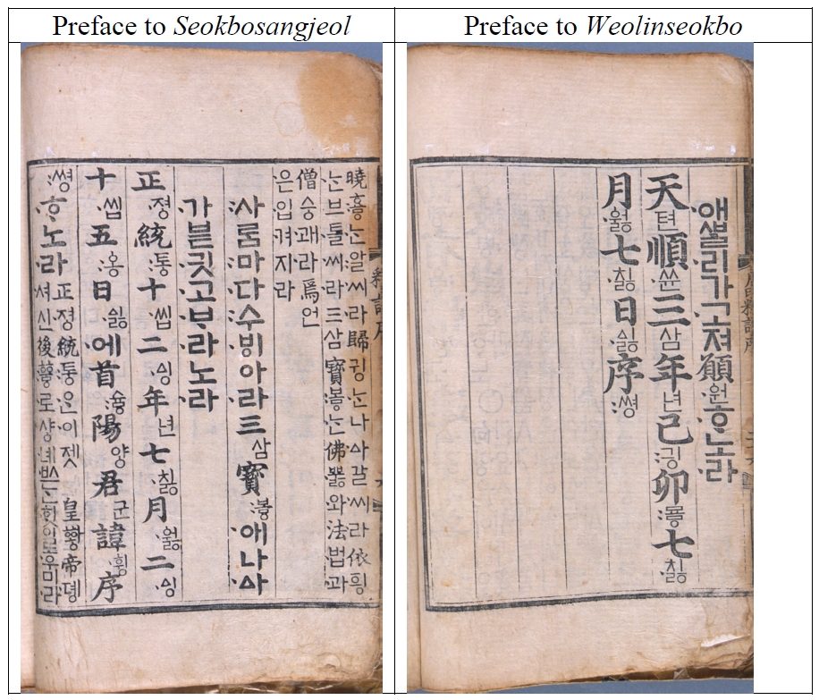
Figure 2The first and last pages of Daemyeongyeongryeoljeon
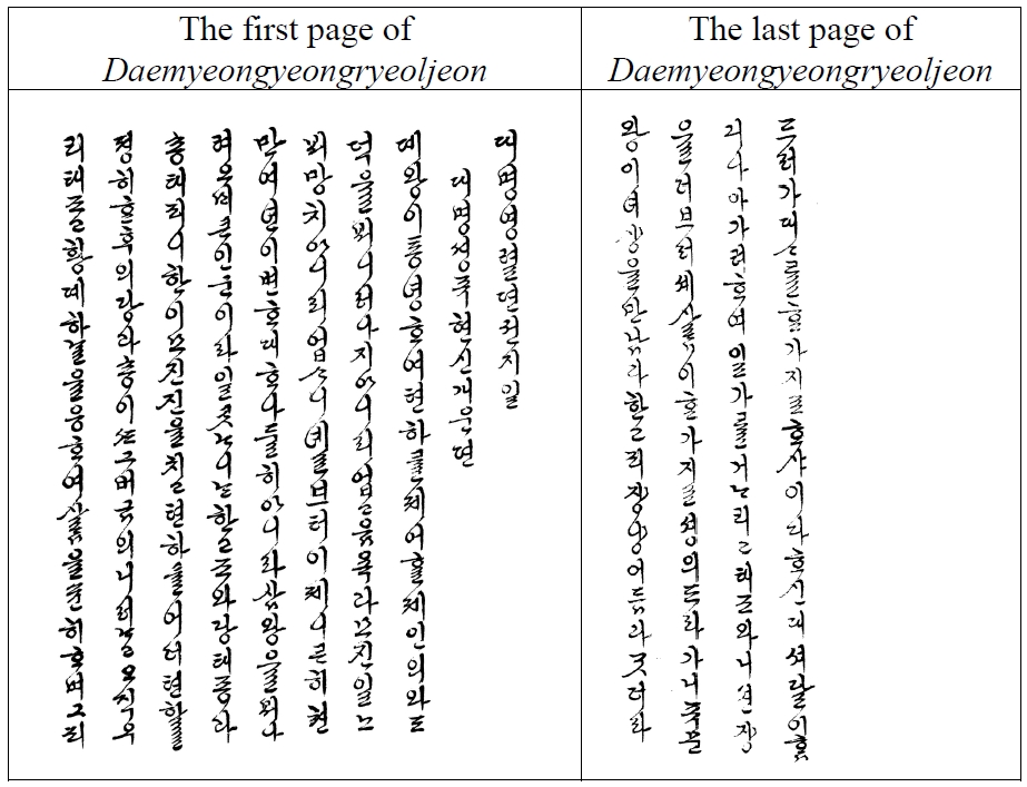
Figure 3Linguistic clues indicating the dates in Seokbosangjeol, and Gomunjinbo Eonhae
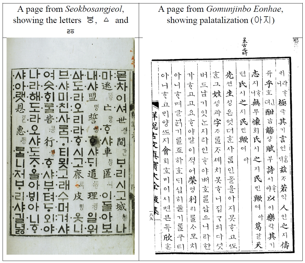
Figure 4Architecture of the bag-of-words unigram model
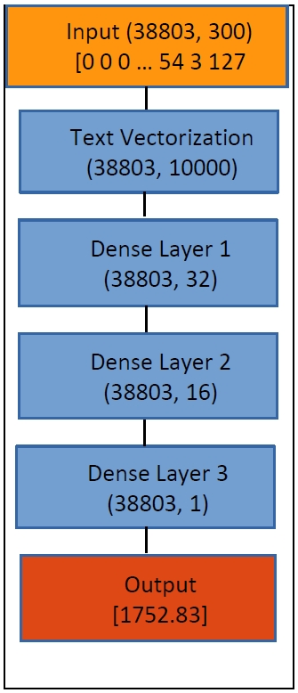
Figure 5Loss during training of the Bag-of-words
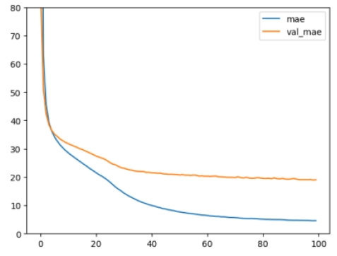
Figure 6Loss during training of the regularized Bag-of-words unigram model
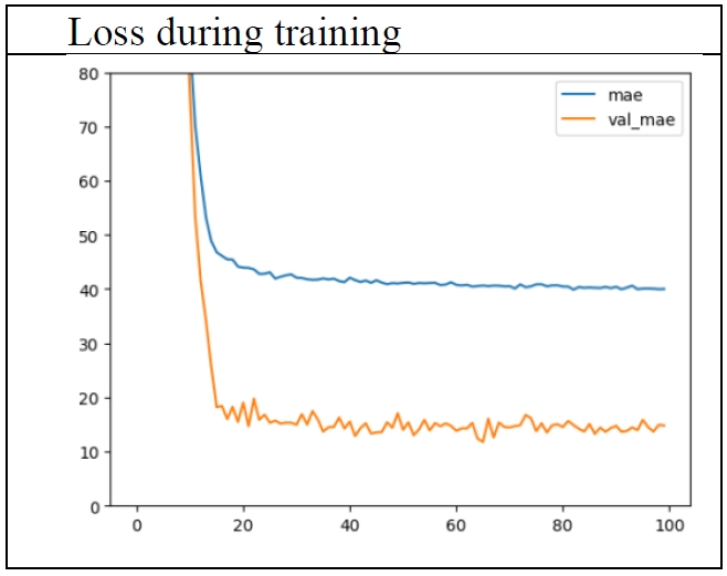
Figure 7Loss during training of the power-increased Bag-of-words unigram model
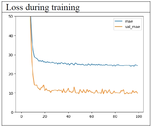
Figure 8Loss during training of the bag-of-words bigram model
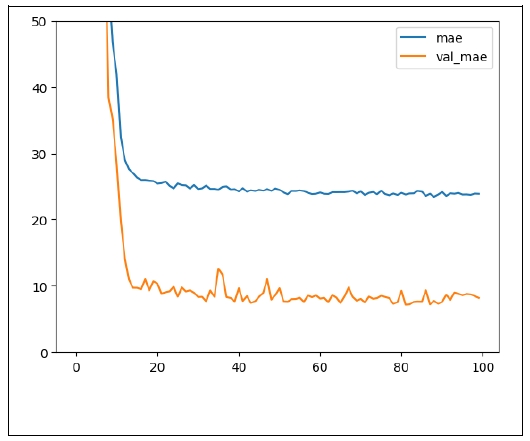
Figure 9Architecture of the CNN model
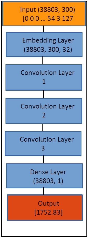
Figure 10Loss during training of the CNN model
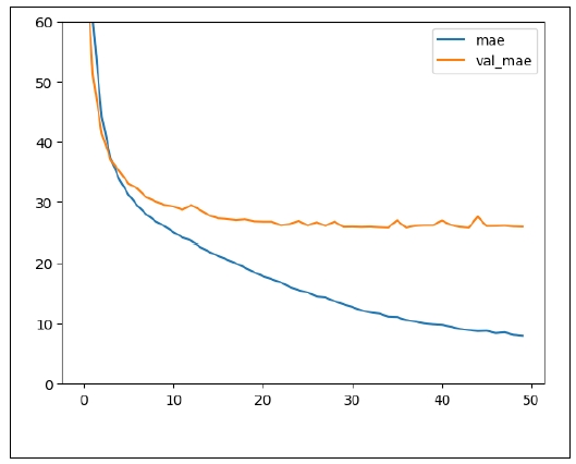
Figure 11Architecture of the RNN model
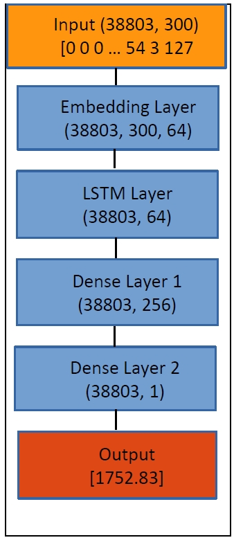
Figure 12Loss during training of the RNN model
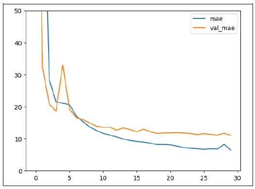
Figure 13Loss during training of the Transformer model
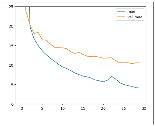
Figure 14Heatmap showing the activation level of each pixel of an image
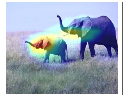
Figure 15Plots showing heat score vs. frequency
Figure 16Histograms by the LSTM model
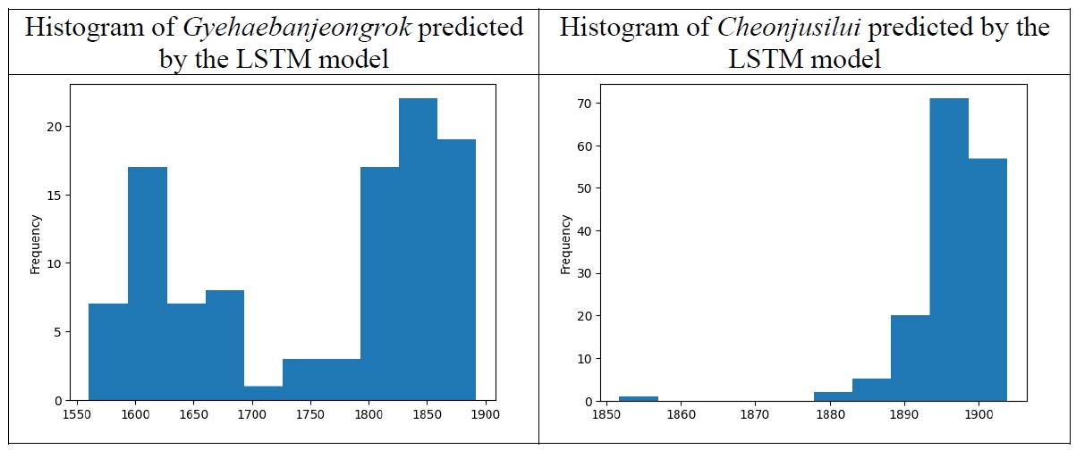
Figure 17Histograms by the Transformer model
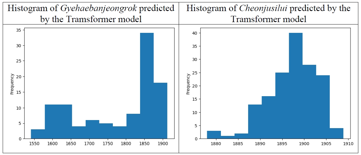
Table 1.Trade-off between the length of a sample and the number of samples
Table 1.
|
Length of a sample |
# of samples |
Training set (64%) |
Validation set (16%) |
Test set (20%) |
|
100 |
145,700 |
93,248 |
23,312 |
29,140 |
|
200 |
72,850 |
46,624 |
11,656 |
14,570 |
|
300 |
48,504 |
31,042 |
7,761 |
9,701 |
|
350 |
41,605 |
22,627 |
6,657 |
8,321 |
|
400 |
36,425 |
23,312 |
5,828 |
7,285 |
Table 2.Loss of the Bag-of-words unigram model
Table 2.
|
MSE (years squared) |
MAE (years) |
|
Training set |
55.65 |
4.60 |
|
Validation set |
1332.23 |
19.06 |
|
Test set |
1579.12 |
20.68 |
Table 3.Loss of the regularized Bag-of-words unigram model
Table 3.
|
MSE (years squared) |
MAE (years) |
|
Training set |
2769.32 |
40.62 |
|
Validation set |
585.44 |
11.79 |
|
Test set |
827.23 |
15.85 |
Table 4.Loss of the power-increased Bag-of-words unigram model
Table 4.
|
MSE (years squared) |
MAE (years) |
|
Training set |
1080.93 |
24.94 |
|
Validation set |
489.35 |
10.01 |
|
Test set |
712.51 |
11.40 |
Table 5.Loss of the bag-of-words bigram model
Table 5.
|
MSE (years squared) |
MAE (years) |
|
Training set |
1036.47 |
24.09 |
|
Validation set |
392.33 |
7.19 |
|
Test set |
482.18 |
8.54 |
Table 6.
Table 6.
|
MSE (years squared) |
MAE (years) |
|
Training set |
568.11 |
16.03 |
|
Validation set |
1752.27 |
26.32 |
|
Test set |
2111.83 |
27.10 |
Table 7.
Table 7.
|
MSE (years squared) |
MAE (years) |
|
Training set |
103.44 |
6.80 |
|
Validation set |
575.09 |
11.26 |
|
Test set |
649.61 |
11.60 |
Table 8.Loss of the Transformer model
Table 8.
|
MSE (years squared) |
MAE (years) |
|
Training set |
80.84 |
5.45 |
|
Validation set |
594.07 |
10.56 |
|
Test set |
698.46 |
10.84 |
Table 9.Unigram graphemes with the highest normalized heat scores
Table 9.
|
Table 10.Bigram graphemes with the highest normalized heat scores
Table 10.
|
Table 11.Ground truth and predicted years of the documents of the 15th century
Table 11.
|
title |
year |
pred |
|
0 |
석보상절03 |
1447 |
1444.26123 |
|
1 |
석보상절03 |
1447 |
1449.315063 |
|
2 |
석보상절03 |
1447 |
1464.890869 |
|
3 |
석보상절03 |
1447 |
1447.827393 |
|
4 |
석보상절03 |
1447 |
1434.583618 |
|
... |
... |
... |
... |
|
6464 |
진언권공 |
1496 |
1476.577759 |
|
6465 |
진언권공 |
1496 |
1530.682373 |
|
6466 |
진언권공 |
1496 |
1498.449951 |
|
6467 |
진언권공 |
1496 |
1485.773193 |
|
6468 |
진언권공 |
1496 |
1499.771729 |
|
6469 rows × 3 columns |
Table 12.Predictions and standard deviations of the LSTM model
Table 12.
|
Dates of the Jangseogak documents predicted by the LSTM model |
Standard deviations of predicted dates per each document |
|
pred
|
열성지장통기 |
1728.978923 |
|
pred
|
|
title
|
|
열성후비지문 |
1743.873079 |
title
|
|
|
계해반정록 |
1755.16872 |
완월회맹연 |
1836.439343 |
천주실의 |
5.623350 |
|
고문백선 |
1813.535319 |
유씨삼대록 |
1817.196457 |
실록초본 |
9.907878 |
|
국조고사 |
1794.245642 |
유이양문록 |
1840.931107 |
선보잡락언해 |
13.722932 |
|
낙성비룡 |
1775.297715 |
윤하정삼문취록 |
1848.837982 |
임신평난록 |
21.163782 |
|
명행정의록 |
1846.645625 |
임신평난록 |
1866.658294 |
한조삼성기봉 |
30.573881 |
|
무오연행록 |
1841.143464 |
정미가례시일기 |
1835.123678 |
엄씨효문청행록 |
32.308008 |
|
벽허담관제언록 |
1848.944505 |
조야기문 |
1750.045986 |
윤하정삼문취록 |
33.930213 |
|
병자록 |
1743.86153 |
조야첨재 |
1828.512066 |
명행정의록 |
36.441314 |
|
사문대의록 |
1765.28703 |
조야회통 |
1828.990723 |
벽허담관제언록 |
37.182772 |
|
산성일기_병자 |
1783.439747 |
학석집(한글) |
1878.469922 |
유이양문록 |
37.575597 |
|
선보잡락언해 |
1888.506897 |
한조삼성기봉 |
1859.522524 |
...... |
|
선택요람 |
1853.460227 |
현몽쌍룡기 |
1831.715601 |
열성지장통기 |
80.957604 |
|
선부군언행유사 |
1766.100093 |
홍경내전 |
1781.141518 |
선부군언행유사 |
81.263283 |
|
신미록 |
1791.836272 |
화씨충효록 |
1836.499052 |
열성후비지문 |
81.842455 |
|
실록초본 |
1890.142447 |
화정선행록 |
1831.80543 |
조야기문 |
82.426335 |
|
엄씨효문청행록 |
1851.211567 |
천주실의 |
1896.516627 |
병자록 |
83.255140 |
|
|
|
|
신미록 |
91.391200 |
|
|
|
|
홍경내전 |
104.377288 |
|
|
|
|
계해반정록 |
110.574844 |
Table 13.Predictions and standard deviations of the Transformer model
Table 13.
|
Dates of the Jangseogak documents predicted by the LSTM model |
Standard deviations of predicted dates per each document |
|
pred
|
열성지장통기 |
1774.778172 |
|
pred
|
|
title
|
|
열성후비지문 |
1781.626921 |
title
|
|
|
계해반정록 |
1776.894681 |
완월회맹연 |
1850.06383 |
천주실의 |
5.582687 |
|
고문백선 |
1820.294533 |
유씨삼대록 |
1843.345866 |
실록초본 |
9.633203 |
|
국조고사 |
1830.799083 |
유이양문록 |
1864.132671 |
선보잡락언해 |
11.201670 |
|
낙성비룡 |
1802.047043 |
윤하정삼문취록 |
1855.230312 |
임신평난록 |
23.407985 |
|
명행정의록 |
1862.019467 |
임신평난록 |
1868.725029 |
한조삼성기봉 |
27.563781 |
|
무오연행록 |
1843.966993 |
정미가례시일기 |
1794.487139 |
윤하정삼문취록 |
33.265788 |
|
벽허담관제언록 |
1867.81161 |
조야기문 |
1764.18373 |
명행정의록 |
33.336713 |
|
병자록 |
1767.580819 |
조야첨재 |
1849.432562 |
엄씨효문청행록 |
34.391305 |
|
사문대의록 |
1767.979588 |
조야회통 |
1855.332041 |
벽허담관제언록 |
34.903389 |
|
산성일기_병자 |
1776.561644 |
학석집(한글) |
1877.044336 |
유이양문록 |
38.701650 |
|
선보잡락언해 |
1900.322198 |
한조삼성기봉 |
1873.623453 |
...... |
|
선택요람 |
1817.476385 |
현몽쌍룡기 |
1850.699927 |
사문대의록 |
82.510204 |
|
선부군언행유사 |
1810.446473 |
홍경내전 |
1834.164509 |
병자록 |
82.621584 |
|
신미록 |
1818.575 |
화씨충효록 |
1856.086874 |
홍경내전 |
84.433661 |
|
실록초본 |
1898.757509 |
화정선행록 |
1853.198077 |
신미록 |
84.848653 |
|
엄씨효문청행록 |
1852.775256 |
천주실의 |
1897.263221 |
조야기문 |
84.979514 |
|
|
|
|
열성후비지문 |
89.220922 |
|
|
|
|
정미가례시일기 |
89.991773 |
|
|
|
|
계해반정록 |
110.655007 |
Table 14.LSTM and Transformer models’ predictions on the Jangseogak documents
Table 14.
|
title |
pred |
pred_lstm |
|
0 |
계해반정록 |
1853.388672 |
1821.7692 |
|
1 |
계해반정록 |
1876.112305 |
1856.4450 |
|
2 |
계해반정록 |
1609.185303 |
1618.0725 |
|
3 |
계해반정록 |
1710.976562 |
1600.5903 |
|
4 |
계해반정록 |
1885.3573 |
1891.7070 |
|
... |
... |
... |
... |
|
49474 |
천주실의 |
1893.72644 |
1900.3711 |
|
49475 |
천주실의 |
1896.940674 |
1890.8717 |
|
49476 |
천주실의 |
1887.2854 |
1897.4349 |
|
49477 |
천주실의 |
1897.868408 |
1891.5488 |
|
49478 |
천주실의 |
1889.480225 |
1886.4396 |
|
49479 rows × 3 columns |
REFERENCES
- Bishop, Christopher. 2006. Pattern Recognition and Machine Learning. Springer.
- Bishop, Christopher and Hugh Bishop. 2023. Deep Learning: Foundations and Concepts. Springer.
- Chollet, François. 2022. Deep learning with python, 2nd edition. Manning Publications.
- Géron, Aurélien. 2022. Hands-On Machine Learning with Scikit-Learn, Keras, and TensorFlow: Concepts, Tools, and Techniques to Build Intelligent Systems, 3rd edition. O'Reilly Media.